文章来源

文章来源：Multi-Granularity Distribution Modeling for Video Watch Time Prediction via Exponential-Gaussian Mixture Network

CODE：https://github.com/BestActionNow/EGMN

Introduction

Motivation

why to predict watch time of videos?

Short-video platforms such as TikTok and KuaiShou have experienced a significant surge in popularity over recent years. These services typically employ a continuous swipe-based streaming play pattern without the need to click through multiple candidates explicitly. Within this paradigm, watch time has emerged as a fundamental indicator of user satisfaction. Therefore, accurate watch time prediction is crucial [40, 43, 44], as it empowers the platform to recommend videos that better align with user interests and ultimately enhance user engagement

抖音 快手短视频 通过划拉视频的播放模式，而不是传统的在多个视频当中选一个，这种情况下 在单个视频上停留的时长成为了用户满意度、参与度评估的重要指标，准确预测视频的观看时长能更好的推荐符合用户偏好的视频，进而提升用户参与度

research gap

任务定义：The watch time prediction is fundamentally a regression problem since its values are continuous and span a wide range. It is well-known that the distribution of labels significantly influences the difficulty of the regression task, where appropriate distribution assumptions can enhance regression accuracy

看到这句话真的泪目，当你拿到一个标签分布特别不均衡的回归任务，真的是谁做谁想哭，都是泪

However, the distribution of short-video watch time remains insufficiently explored. To bridge this knowledge gap, we thoroughly investigate the distribution of short-video watch time using our real-world industrial recommendation data. （要是有真实数据就太香了，很多时候都是在别人公开的部分小数据上run，没机会去探索这个真实分布）

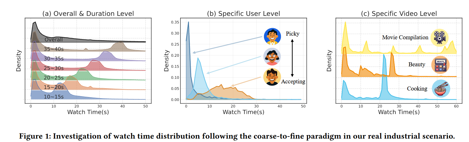
下面最精华的部分来了，在数据集上统计了数据的观看时长分布，图的信息量极大

• Overall Level: We examine the overall distribution of watch time, which reveals pronounced skewness around zero, as shown in the top line of Figure 1(a) 的overall 那个曲线. 表明：users quickly lose interest and swipe away the video. 大部分用户看了开头就退出

• Duration Level: Figure 1(a) 除overall 之外的其它曲线 also presents the distribution at the duration level, where a bimodal pattern（双峰） is observed across different duration groups. 按照视频时长划分视频 。 实际当中对于一个视频 大部分不感兴趣的会在开头退出，对应第一个峰，度过第一个峰之后能筛选出一部分感兴趣的人会持续观看大部分，对应第一个峰和第二个峰之间的区域，下一阶段前可能是了解了视频的大致内容，知道是不是符合自己的需求，或者需求已经满足，所以第二个峰到来（退出观看），然后第二个峰之后陆续的退出，对应坚持刷到结尾

• Specific User Level: We analyze the watch time distribution of specific users as shown in Figure 1(b), which demonstrates notable diversity on such a fine granularity. Some users are rather picky（挑剔的）, quickly swiping past videos until finding one of interest, resulting in a higher skewness of their watch time distribution. Conversely, some users are more accepting, tending to watch each system-recommended video with greater patience, leading to a lower skewness. 这里应该是按照相同视频对不同用户群体进行分析

• Specific Video Level: The watch time distribution of different videos demonstrates a multimodal phenomenon, 这里是指多峰分布，不是多模态 and the differences between videos are even more pronounced. Figure 1(c) provides three representative examples. The cooking video exhibits a bimodal distribution: disinterested users exit early, whereas engaged viewers complete the content. The beauty video’s engagement drives not only partial/full views but also notable replays, yielding a trimodal pattern. In contrast, the movie compilation’s segmented structure features common exit points at scene transitions, ultimately manifesting a multimodal distribution.

we distill two critical challenges for short-video watch time prediction :

• Coarse-grained distribution skewness arises from a substantial concentration of quick-skips, which requires specialized modeling approaches capable of addressing this localized clustering phenomenon. 粗粒度分布稀疏性，即pronounced skewness around zero
• Fine-grained distribution diversity introduces cross-granular incompatibility that amplifies prediction complexity, demanding adaptive architectures to capture heterogeneous characteristics. 细粒度分布差异性，即不同主题+不同人群叠加下的差异

Existing watch time prediction methods typically circumvent these challenges through two principal approaches.

• The first approach is label normalization [45–47], which not only simplifies the label distribution for easier fitting but also provides an unbiased reflection of user interest. However, it may lead to a loss of absolute watch time information, resulting in reduced prediction accuracy.
• The second approach is task transformation [21, 35], where the regression task is transformed into a series of classifications. The benefit is that each subclassification task is easier to learn than the overall regression problem, while the process of discretization and subsequent reconstruction inevitably introduces additional errors

The proposed method

To reconcile distributional discrepancies across different granularities, we assume that short-video watch time is governed by a latent mixture model, formally defined as the Exponential-Gaussian Mixture distribution (EGM distribution), where the exponential component addresses coarse-grained distribution skewness and the Gaussian components adaptively capture fine-grained distribution diversity.

To estimate the parameters of EGM distribution, we propose the corresponding Exponential-Gaussian Mixture Network (EGMN) model using a neural network architecture.

• Initially, we generate a hidden representation shared across all distribution components. Subsequently, the parameters of each distribution component are estimated based on the hidden representation, and a gated network is applied to perform the weighted mixing of multiple distributions.

  上来先估计数据的分布情况，然后 gated network 去分配不同分布的权重？

• A combination of loss functions is used to optimize our model, each addressing different aspects of the prediction task.

• Ultimately, EGMN produces a parameterized instance of EGM distribution in an end-to-end manner and uses its expected value as the final prediction.

Through extensive experiments, we demonstrate the superiority of EGMN compared to existing state-of-the-art methods. Moreover, we design an ablation study to validate the distributional assumptions and quantify the contribution of each component to our loss function. Comprehensive experimental results have proven that EGMN exhibits an excellent distribution-fitting ability across coarse-to-fine-grained levels. Remarkably, EGMN successfully captures the latent interaction effects between user preferences and video characteristics, which are crucial for recommender systems. In summary, the major contributions of this paper are as follows:

• (1) Based on our observations of short-video watch time distribution at various granularities, we introduce a well-founded distributional assumption: EGM distribution, which is compatible with the distribution characteristics of each granularity.
• (2) To parameterize EGM distribution, we propose EGMN for watch time prediction, which simultaneously models the concentrated characteristics of quick-skips and captures the latent viewing patterns arising from user-video interactions.
• (3) Extensive experiments are conducted on both offline datasets and the online short-video feeding scenario of Xiaohongshu App, demonstrating that EGMN significantly outperforms existing state-of-the-art methods.

RELATED WORK

Existing works related to watch time prediction:

• This mismatch between modeling assumptions and empirical data can lead to suboptimal predictions：traditional approaches to regression-based watch time prediction rely on specific assumptions on label distribution or error distribution. Such as Value Regression (VR) evaluated via Mean Squared Error (MSE) assumes that the watch time conform to the normal distribution, which is violated in real-world scenarios. Watch time data typically follows a highly skewed, long-tailed distribution, with most data being short and only a few lasting significantly longer. Weighted Logistic Regression (WLR)[6] fits a weighted logistic regression model, where click samples are weighted by watch-time and unclick samples receive unit weight. Due to the lack of explicit click behaviors in streaming short-video platforms, WLR can not be directly applied to our system.
• Recent research has shifted focus toward watch time debiasing, aiming to extract unbiased user interests from noisy observations. For example, D2Q[45] mitigates duration bias in watch time prediction by reformulating the task as a quantile regression problem, where videos are first partitioned into discrete duration-based bins, and a regression model is trained for each group to estimate its conditional watch time distribution。Although this approach effectively addresses systemic biases across duration, its reliance on hard grouping introduces fundamental limitations. By enforcing rigid duration boundaries, D2Q fails to capture finer-grained behavioral patterns and produces discontinuous predictions across bin edges. 对于切片边界的数据，预测表现不佳
• Another line of work, such as D2CO[47], identifies noisy watching behavior as a confounding factor that distorts true engagement signals. While D2CO employs a Gaussian Mixture Model (GMM) to separate meaningful watch time from noise, it fails to account for the rich diversity in user-video interactions, such as quick-skips, replays. Meanwhile, CWM[46] points out that the duration bias is derived from the truncation of the user’s theoretical maximum watch time by video duration and a cost-based correction function is defined to transfer original watch time into an unbiased regression space. However, CWM’s duration truncation neglects replay behaviors, and the transformation of original watch time may cause distribution information loss. 没太懂 后续继续研究
• Alternatively, some methods reformulate watch time prediction as a series of classification tasks, preserving ordinal relationships between different watch time. TPM[21] leverages a tree-based probability model to capture conditional dependencies between these classifications, improving hierarchical reasoning. Given the highly imbalanced nature of watch time data, CREAD[35] conducts a systematic study on how discretization granularity affects both model learning and prediction restoration. It proposes an error-adaptive discretization mechanism to balance bias and variance, yet it lacks deeper analysis of fine-grained patterns.
• Finally, GR[22] presents a Generative Regression framework capable of modeling watch time alongside other continuous variables. GR reformulates watch time prediction as a sequence generation task and offers a more flexible and expressive approach

Method

Problem Definition

Let $ x \in \mathbb{R}^d $ represent the embedded feature vector for a user-video pair, incorporating user features, video features, and context information, while $ t \in \mathbb{R}^+ $ represent the watch time. Watch time prediction aims to find a function $ f (·) : \mathbb{R}^d \to \mathbb{R}^+ $, such that the discrepancy between the predicted outputs $ f (x) $ and the ground truth $ t $ is minimized under certain metrics. Previous approaches typically select a specific metric (e.g. MSE) to construct the loss function between $ f (x) $ and $ t $, and then optimize $ f (·) $ through parameter estimation. However, these metrics rely on oversimplified assumptions on the watch time probability distribution $ p (t) $ and ignore the inherent heterogeneity across multi-granularity levels, which motivates our probabilistic modeling of $ p (t) $ instead of arbitrary function optimization.

这段文字清晰地定义了一个监督学习问题：

• 输入向量 (Input Vector): $ x \in \mathbb{R}^d $
  • 这是一个代表用户-视频对的嵌入特征向量。
  • 它融合了三类信息：
    1. 用户特征 (如：年龄、历史兴趣)
    2. 视频特征 (如：类别、标签、时长)
    3. 上下文信息 (如：时间、设备、地理位置)
• 输出值 (Output Value): $ t \in \mathbb{R}^+ $
  • 这是一个正实数，代表观看时长。
• 目标 (Goal): 找到一个函数 $ f(\cdot) $，使得预测值 $ f(x) $ 和真实值 $ t $ 之间的差异最小化。

简单总结： 这是一个回归问题，旨在利用丰富的特征来预测用户观看一个视频的时长。

---

传统方法存在的问题：

1. 依赖于过度简化的分布假设

• 传统做法： 直接选择一个损失函数（如 MSE）来度量 $ f(x) $ 和 $ t $ 的差异。
• 隐含的、过度简化的假设：
  • 使用 MSE 等价于假设误差 $ \epsilon = t - f(x) $ 服从均值为零的正态分布。
  • 这进而暗示着观看时长 $ t $ 本身在其均值 $ f(x) $ 附近也服从正态分布。
• 现实情况： 观看时长的真实分布 $ p(t) $ 通常不是正态的。它可能具有以下特性：
  • 高度偏斜 (Heavily Skewed): 大量短观看，少量长观看。
  • 零值聚集 (Zero-inflated): 很多用户点开即离开，观看时间为零。
  • 长尾分布 (Long-tailed): 存在少数持续时间非常长的观看。
• 结论： 强行使用基于特定分布假设的损失函数，在统计上是”不正确的”，会导致模型在有偏数据上表现不佳。

2. 忽略了多粒度级别的内在异质性

• “异质性” (Heterogeneity): 指数据不是同质的，不同用户群体或视频类型的行为模式差异很大。
• “多粒度级别” (Multi-granularity Levels): 数据可以从不同层次观察：
  • 用户粒度: 有的用户是”速览者”，只看几秒；有的是”深度观看者”。
  • 视频粒度: 短视频和长视频的观看时长分布完全不同。
  • 上下文粒度: 通勤时和晚上在家时的观看行为也不同。
• 传统做法的问题： 一个单一的模型 $ f(\cdot) $ 和损失函数试图用同一套标准拟合所有数据，无法捕捉和适应这种内在的、不同粒度上的行为差异。

---

作者提出的解决方案方向

基于以上批判，作者提出了核心思路：

“…which motivates our probabilistic modeling of $ p(t) $ instead of arbitrary function optimization.”

这实现了一个范式转变：

范式	传统方法 (函数优化)	本文方法 (概率建模)
目标	学习一个映射函数 $ f: x \to t $	学习一个条件概率分布 $ p(t | x) $

这个转变带来的巨大优势：

1. 更丰富的输出 (Richer Output):
   • 模型输出的不是单个值，而是关于观看时长 $ t $ 的完整概率分布。
   • 我们不仅可以得到点估计（如分布的均值），还可以得到不确定性（如方差、分位数）。
2. 摆脱单一损失函数的束缚 (Freedom from Arbitrary Loss):
   • 一旦建模了 $ p(t | x) $，就可以使用极大似然估计 (Maximum Likelihood Estimation) 来训练模型。
   • 我们只需要选择一个能真实反映观看时长分布形态的概率模型（例如，指数分布、伽马分布、混合模型），而不再需要纠结于选择MSE或MAE这类”任意”的损失函数。
3. 自然处理异质性 (Natural Handling of Heterogeneity):
   • 概率模型可以设计得非常灵活。模型可以自动学习到：
     • 对于”速览者”用户，$ p(t | x) $ 是一个集中在短时间的分布。
     • 对于”深度观看者”，$ p(t | x) $ 是另一个集中在长视频的分布。
   • 这就在一个统一的概率框架内，自然地刻画了多粒度的异质性。

---

总结对比

方面	传统方法	本文方法
目标	找到一个函数 $ f(x) \approx t $	找到一个条件分布 $ p(t | x) $
核心假设	误差分布简单（如正态）	观看时长本身的分布 $ p(t) $ 复杂，需精确建模
如何处理异质性	难以处理，用一个模型拟合所有数据	易于处理，通过概率分布的形状变化来适应不同群体
训练准则	最小化任意选择的损失函数（如MSE）	最大化似然函数，基于对 $ p(t) $ 的合理概率假设

最终结论： 这段文字的核心理念是主张从一种机械的、基于简单距离度量的函数拟合思路，转向一种基于数据生成机制的概率生成思路。后者在统计上更严谨，对复杂现实数据的建模能力更强，并能提供更丰富的预测信息。

An Empirical Assumption to $ p (t)$

we assume that $ p (t)$ follows a latent EGM distribution as a mixture of one exponential distribution and K Gaussian distributions, whose density function is formulated as:

基本思想：这是一个混合模型，通过将多个简单的概率分布加权组合，来建模复杂的真实数据分布 \(p(t) = \omega_0 f_{\text{exp}}(t|\lambda) + \sum_{k=1}^K \omega_k f_{\text{gauss}}(t|\mu_k, \sigma^2_k) \tag{1}\)

1. 各分量说明

(1) 指数分布分量

• 函数形式： $ f_{\text{exp}}(t

  \lambda) = \lambda e^{-\lambda t} $

• 分布特性：
  • 描述持续时间短、迅速衰减的行为模式
  • 适用于建模”快速跳过”或”短暂观看”的行为
  • 概率密度在 $ t=0 $ 附近最高，随时间指数衰减

(2) 高斯分布分量

• 函数形式： $ f_{\text{gauss}}(t

  \mu, \sigma^2) = \frac{1}{\sqrt{2\pi\sigma^2}} e^{-\frac{(t-\mu)^2}{2\sigma^2}} $

• 分布特性：
  • 描述集中在特定时长范围的观看行为
  • 每个高斯分量可以捕捉一种”典型”的观看模式
  • 通过多个高斯分量（$ K $ 个）可以建模多峰分布

2. 混合权重

• 权重约束： $ \sum_{k=0}^K \omega_k = 1 $
• 物理意义：
  • $ \omega_0 $：用户进行”快速跳过”行为的概率
  • $ \omega_k $ ($ k=1,…,K $)：用户属于第 $ k $ 种典型观看模式的概率

Here, we present the assumed distribution selection rationale. The components of EGM distribution are carefully selected based on the observed characteristics of watch time distribution:

• (1) Exponential Component: At the coarse-grained level, the distribution is highly skewed, with a significant concentration of quick-skips. The exponential distribution is well-suited for modeling the quick-skipping behavior due to its memoryless property and concentration of probability mass near zero [1].
• (2) Gaussian Components: At the fine-grained level, the distribution becomes more intricate. Users with diverse viewing habits interact with various types of videos, resulting in a spectrum of latent consumption patterns. Given that Gaussian mixture distributions have been theoretically established as statistically consistent estimators for complex multimodal distributions [26, 50], we leverage them to effectively capture diversity in user preferences and video characteristics.

我们发现，用户的观看时长很复杂，不能用一个简单的规律来描述。于是我们把这个问题拆成两部分来看：一部分是“随便看看”，另一部分是“认真看完”，并分别用不同的数学工具来建模。

想象一下，你是一个视频平台的经理，想研究用户看视频的习惯。你调出数据一看，发现情况非常复杂：

1. 第一类用户：“点开就关”族（对应指数分布）

• 你观察到的现象： 有非常多的用户，点开一个视频，只看几秒钟就关掉了。在数据图上，这些超短的观看时长密密麻麻地堆在起点附近。
• 我们怎么建模： 对于这种“秒退”行为，我们选用了一个叫 “指数分布” 的模型。
  • 为什么用它？ 因为它有两个特别符合现实的特性：
    • “秒忘”特性： 一个用户下一秒会不会关掉视频，和他已经看了多久没关系。他可能看3秒后关，也可能看10秒后关，决策很随机。这个模型不“记仇”，正好能描述这种随机性。
    • “扎堆在零”：这个模型的形状，天生就是大部分数据都挤在“零时长”附近，完美匹配我们看到的“大量快速跳过”的现象。

简单说：我们用“指数分布”来代表那些“缺乏耐心、点开就走”的用户。

2. 第二类用户：“各种看完”族（对应高斯混合分布）

• 你观察到的现象： 排除了“秒退”用户，剩下的用户行为也各不相同，形成了好几个“小团体”：
  • 小团体A： 喜欢看短视频，集中在1-3分钟。
  • 小团体B： 喜欢看中视频，集中在5-15分钟。
  • 小团体C： 是深度用户，看长视频，集中在20-40分钟。
  • 数据图上会呈现出好几个“小山包”。
• 我们怎么建模： 对于这种“百花齐放”的观看模式，我们选用了一个叫 “高斯混合模型” 的工具。
  • 为什么用它？ 因为它就像一个 “万能橡皮泥”：
    • 它可以同时捏出好几个“小山包”，每个“小山包”（一个高斯分布）代表一类典型的观看习惯（比如爱看短视频的、爱看长视频的）。
    • 它在数学上被证明，只要“小山包”足够多，就能模拟出任何奇奇怪怪的复杂形状。所以用它来捕捉用户偏好和视频类型的多样性，非常强大和有效。

简单说：我们用“高斯混合模型”这个万能橡皮泥，来捏出那些“有不同观看偏好和习惯”的用户群体

Our Approach: EGMN

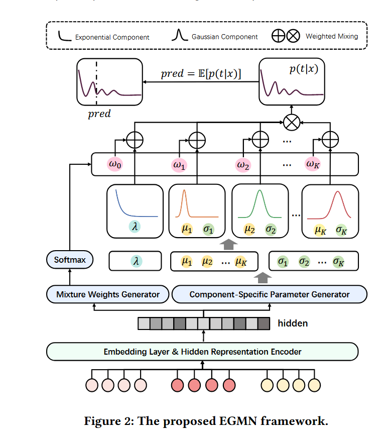
In this section, we propose a model EGMN for the parameterization of the EGM distribution as illustrated in Figure 2. Specifically, we employ a deep feed-forward network [2, 17, 31] that takes the feature vector x as input and estimates the parameters of EGM distribution.

Hidden Representation Encoder

For each user-item pair, we collect features from multiple sources:

• User features: demographic information, historical behavior patterns, and engagement statistics
• Video features: content characteristics, duration, category, and creator information
• Contextual features: time of day, weekday patterns and device type

Available features are processed through embedding layers to create the feature vector x. Initially, x is fed into a feature encoder backbone to obtain a hidden representation $ h $, which is shared across multiple components in EGM distribution where $ g_{backbone} $ can be instantiated with any feature encoding backbone adaptable to recommender prediction scenarios, e.g. DCN [39], DIN [49], SENet [14], Transformer [38], etc. It should be noted that EGMN has the potential to be enhanced by specific model design and feature engineering, since EGMN is proposed as a backbone agnostic paradigm that inherently supports the integration of user segmentation and contextual signals. \(h = g_{backbone} (x)\)

Mixture Parameter Generator

核心功能

混合参数生成器是整个模型的核心部件。它的任务是：将神经网络提取的隐藏特征表示 \(h\)，转化为一个定制化的混合概率分布的所有参数。这意味着，对于不同的输入 \(x\)，它会动态地生成不同的分布参数。

---

参数生成分支

隐藏表示 \(h\) 被送入四个独立的分支，分别计算以下参数：

1. 指数分布速率参数

\[λ(x) = \text{softplus}(W_λ h + b_λ) \tag{3}\]

• 功能：确定“快速跳过”行为的普遍程度。
• 使用 Softplus 激活函数的原因：确保速率 \(λ\) 始终为正值（速率必须为正数）。

2. 高斯分布均值参数

\[μ_k (x) = \frac{1}{λ(x)} + \text{softplus}(W_{μ_k} h + b_{μ_k}) \quad \text{for } k ∈ \{1, \ldots, K\} \tag{4}\]

• 功能：确定每个高斯分量对应的“典型观看时长”。
• 设计精妙之处：强制每个高斯分布的均值都大于指数分布的均值（\(1/λ(x)\) 是指数分布的均值）。
• 目的：确保模型可辨识性，防止分量混淆。明确分工为：指数分量专门捕捉靠近零点的短时长行为，高斯分量则捕捉更长的、多样的观看模式。

3. 高斯分布方差参数

\[σ^2_k (x) = \text{softplus}(W_{σ_k} h + b_{σ_k}) \quad \text{for } k ∈ \{1, \ldots, K\} \tag{5}\]

• 功能：控制每个高斯分布“钟形曲线”的宽窄。方差大，说明这类用户的观看时长很分散；方差小，说明他们的观看时长很集中。

4. 混合权重参数

\[[ω_0 (x), ω_1 (x), \ldots, ω_K (x)] = \text{softmax}(W_ω h + b_ω) \tag{6}\]

• 功能：决定“快速跳过”（对应 \(ω_0\)）和每一种“典型观看模式”（对应 \(ω_1\) 到 \(ω_K\)）各自占多大比重。
• 使用 Softmax 激活函数的原因：保证所有权重之和为 1，形成一个合法的概率分布。

---

激活函数的选择

Softplus：\(\text{softplus}(z) = \log(1 + e^z)\) 用于速率、均值、方差，确保这些参数为正。

Softmax：用于混合权重，确保所有权重非负且和为 1。

可学习参数: 公式中的 \(W_*\) 和 \(b_*\) 是线性变换层的权重和偏置，在模型训练过程中通过梯度下降进行学习。

---

To ensure identifiability and prevent component ambiguity, we constrain the mean of the Gaussian component to exceed that of the exponential component in Equation (4). This configuration allows the exponential component to explicitly model the skewed density near zero, while the Gaussian components capture complex multimodal patterns in the mixture distribution.

Following the formulation in Equation (1), the complete mixture distribution conditioned on the input features is defined as:

将所有生成的参数代入，得到条件混合分布的最终形式： \(p(t | x) = ω_0(x) f_{\text{exp}}(t | λ(x)) + \sum_{k=1}^{K} ω_k(x) f_{\text{gauss}}(t | μ_k(x), σ^2_k(x)) \tag{7}\)

混合参数生成器实现了一个从抽象特征到具体概率分布的映射：

1. 动态定制：对于每一个输入样本 \(x\)，都生成一套独有的分布参数，实现了个性化预测。
2. 明确分工：通过数学约束，让指数分量和高斯分量各司其职，分别捕捉数据中“短时长偏斜”和“多峰复杂”的特性。

3. 概率输出：模型的最终输出不是一个单一值，而是一个完整的概率分布 $$ p(t

   x) $$，这为决策提供了丰富的信息（如预测不确定性、各种可能性的概率等）。

这标志着模型从传统的“点预测”范式，彻底转向了更强大、更灵活的“概率预测”范式。

Training Objective

我们使用一种组合损失函数来优化EGMN模型，其中的每一种损失函数都针对预测任务的不同方面进行优化。

1. 最大似然估计损失

最大似然估计损失是我们的主要目标函数。其核心思想是：调整模型参数，使得模型预测出的概率分布下，我们观测到的真实观看时长数据出现的“可能性”达到最大。

损失函数定义

\[\mathcal{L}_{MLE} = -\frac{1}{N} \sum_{i=1}^{N} \log \, p(t_i | x_i) \tag{8}\]

公式解读：

• $ N $：训练样本的总数。
• $ t_i $：第 $ i $ 个样本的真实观看时长。
• $ x_i $：第 $ i $ 个样本的输入特征向量。

• $ p(t_i

  x_i) $：我们的EGM模型根据特征 $ x_i $ 预测出的概率分布在 $ t_i $ 这一点的概率密度值。

将我们之前定义的混合模型公式 (7) 代入上式，可以得到具体的计算形式：

\[\mathcal{L}_{MLE} = -\frac{1}{N} \sum_{i=1}^{N} \log \left[ \omega_0(x_i) f_{\text{exp}}(t_i | \lambda(x_i)) + \sum_{k=1}^{K} \omega_k(x_i) f_{\text{gauss}}(t_i | \mu_k(x_i), \sigma^2_k(x_i)) \right] \tag{9}\]

计算过程说明：

1. 对于每一个训练样本 $ (x_i, t_i) $，模型通过混合参数生成器输出所有定制化的参数：$ \omega_k(x_i), \lambda(x_i), \mu_k(x_i), \sigma^2_k(x_i) $。
2. 分别计算指数分布 $ f_{\text{exp}} $ 和 K个高斯分布 $ f_{\text{gauss}} $ 在真实值 $ t_i $ 处的概率密度。

3. 将这些密度值用对应的混合权重 $ \omega_k(x_i) $ 进行加权求和，得到混合模型在 $ t_i $ 处的总概率密度 $ p(t_i

   x_i) $。

4. 取该密度的对数，然后取负值，并对所有样本求平均，得到最终的损失 $ \mathcal{L}_{MLE} $。

损失函数的直观作用与意义

• 指导优化过程：这个损失函数通过惩罚那些为真实数据分配低概率的模型预测，同时奖励那些为真实数据分配高概率的预测，来指导模型的优化方向。

• 实现精准捕捉：通过最小化 $ \mathcal{L}_{MLE} $，EGMN模型学习去精确地捕捉在不同内容类型和观看情境下，用户参与模式的底层数据分布。它不仅仅是在学习预测一个单一的数值，而是在学习整个数据生成过程的概率规律。

总结来说，最大似然估计损失确保了我们的模型不仅仅是在进行“点猜测”，而是在学习一个能够反映现实世界复杂性和不确定性的、真正有意义的概率模型。

2. Entropy Maximization Loss.

To prevent the model from collapsing into a single component during training, we introduce an entropy maximization regularization term [48] for the mixture weights:
\(\mathcal{L}_{entropy} = \frac{1}{N} \sum_{i=1}^{N} \sum_{k=0}^{K} \omega_k (x_i) \log \omega_k (x_i) \tag{10}\)

Minimizing this loss is equivalent to maximizing the entropy between weights in $ω (x_i ) $and encourages the model to utilize multiple components when appropriate, rather than assigning all probability mass to a single component. This is crucial for maintaining the model’s ability to capture the multimodal nature of the watch time distribution.

3.Regression Loss

To ensure that our model also performs well on absolute value estimation, we incorporate a regression loss between the expected value of EGM distribution and the actual watch time: \(\mathcal{L}_{reg} = \frac{1}{N} \sum_{i=1}^{N} |t_i - \hat{t}_i| \tag{11}\) (指数分布的期望是 $1/\lambda$，高斯分布的期望是 $\mu$)

where $\hat{t}_i $ is the expectation of $p (t |x)$ \(\hat{t}_i = \mathbb{E}[p(t|x_i)] = \omega_0(x_i) \frac{1}{\lambda(x_i)} + \sum_{k=1}^{K} \omega_k(x_i) \mu_k(x_i) \tag{12}\)

We use $\hat{t}i$ as the final watch time prediction during the evaluation. By minimizing$\mathcal{L}{reg}$, we explicitly optimize EGMN’s ability to generate accurate prediction while maintaining its rich distributional awareness. Together with $\mathcal{L}_{MLE}$ , this triple-objective design ensures that the model remains versatile in both probabilistic modeling and value regression.

4. Combined Loss Function.

The final loss function is a weighted combination of the three individual losses: \(\mathcal{L} = \mathcal{L}_{MLE} + \alpha \mathcal{L}_{entropy} + \beta \mathcal{L}_{reg} \tag{13}\)

where α and β are hyperparameters controlling the relative importance of each objective. It is worth emphasizing that both the uniqueness of mixture model parameters in EGMN and the neural network’s approximation capability to the o

Inference

During inference, EGMN generates complete conditional probability distributions over possible watch time ranges in a fully end-toend manner. This eliminates any need for computational preprocessing or reconstruction steps, making it particularly well-suited for industry deployments where computational efficiency and latency are critical factors. For the standard watch time prediction, we simply utilize the expected value of p (t

x) in Equation (12) as an estimation. Moreover, EGMN has the flexibility to provide additional information:

• Recognition of quick-skipping behaviors.
• Cumulative probability on specific watch time intervals.
• Quantile estimation [25] for specific user or video.
• Statistical confidence for uncertainty quantification [34].
• In industrial recommender systems, this flexibility allows to leverage the same underlying model for diverse strategy designs without requiring specialized model variants.

Experiments

In this section, we conduct extensive experiments and analyses to demonstrate the effectiveness of the EGMN model. In these experiments, five research questions are explored:

• RQ1: How does EGMN perform compared to existing state-of-the-art baselines in the offline/online watch time prediction task?
• RQ2: To what extent can EGMN improve the recognition of quickskipping behaviors compared to conventional approaches?
• RQ3: How does the prior distribution selection contribute to overall effectiveness in predicting watch time?
• RQ4: How does each part of the loss function(Equation (13)) affect the final performance of EGMN?
• RQ5: How does our approach capture coarse-to-fine-grained distribution information in video watch time prediction?

Datasets.

For offline experiments, we evaluate EGMN on a realistic industrial dataset (referred to as Indust) and three public datasets for recommender system. The details of these four datasets are as follows:

• Indust: An industrial dataset sampled from a real-world streaming short-video app with more than 200 million DAUs. We collect interaction logs for 14 days, which contain 951,870 interactions, 2,5947 users, and 7,155 videos. The sampling process ensures the consistency of the watch time distribution between the offline dataset and the online real-time distribution.
• KuaiRec3: A real-world dataset collected from the KuaiShou mobile app recommender logs [10]. It samples 12,530,806 impressions which cover 7,176 users and 10,728 videos. • WeChat4: This dataset is released by WeChat Big Data Challenge 2021, containing impression logs sampled from WeChat Channels within two weeks. It contains 7,310,108 interaction logs between 20,000 users and 96,418 videos.
• CIKM5: A famous dataset sourced from the CIKM16 Cup Competition, is designed to predict user engagement duration in online search sessions. It contains 310,302 sessions and 122,991 items. Although CIKM is not derived from short video recommender systems, we still adopt it to prove the scalability of EGMN.

未完待续,,,,,,

总结与分析

• 将时长预测任务转换为概率分布的参数预测任务，不是直接的去预测y，而是先去预测数据的分布，再预测y
• 学习在实际当中，数据来了之后如何分析数据的规律，得出一个数据分布的假设情况
• 不同主题类似的视频+不同类型的用户群体偏好 会带来复杂的多峰分布（不同场景这个分布规律可能不一样），如何建模。这个问题不仅仅适用于视频平台 对于其它内容平台都有这个特性，就是y得变化，比如变成弹幕数，群体比例

大受震撼！！！！